This article explores the perceptron algorithm, focusing on how it computes rather than how it learns. We will start by briefly mentioning its creator, followed by a close examination how the algorithm works. To conclude, we will add a hidden layer and connect the neurons making a network, that will then implement the non-linear XOR gate.
An idea from the 1950s
Frank Rosenblatt developed the Perceptron in 1958, an early artificial neuron model that mimicked the computational processes of biological neurons.
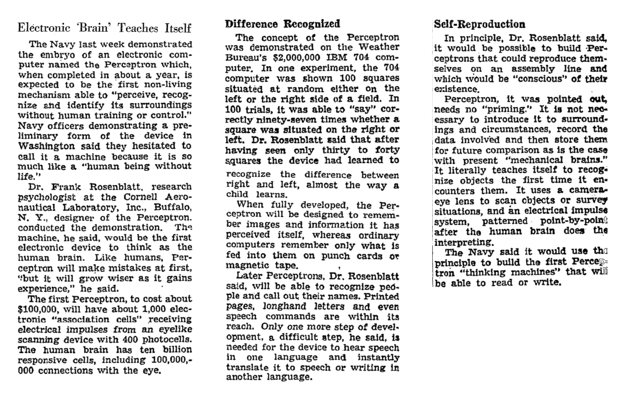
While Rosenblatt was undeniably a visionary, his expectations were somewhat inflated. The promises he made are only now beginning to be fulfilled.
The perceptron algorithm
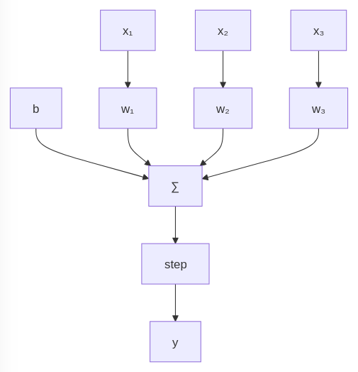
The perceptron works like this:
- Takes 𝑛 inputs of the same size, which can be scalar values or vectors (x₁, x₂, x₃)
- Multiply each input by its own weight, a floating point number (w₁, w₂, w₃)
- Sum the weighted inputs ( ∑ )
- Add a bias term to shift the function, sliding its line to either the left or right on a graph (b)
- Pass the sum through the step function to get the final output (step)
Which can be viewed as:
output = step(dot(x_values, w_values) + b)
Let’s understand each individual component of this computation below.
Dot product
For the weighted summation (simbolized by ∑ on the diagram), we should do:
(x₁ * w₁) + (x₂ * w₂) + (x₃ * w₃)
Let’s take the following values as an example:
| Variable | Value |
|---|---|
| x₁ | 1 |
| x₂ | 2 |
| x₃ | 3 |
| w₁ | 0.1 |
| w₂ | 0.2 |
| w₃ | 0.3 |
This results in:
(1 * 0.1) + (2 * 0.2) + (3 * 0.3) =
0.1 + 0.4 + 0.9
1.4
Since x and w are of equal length, we can use the mathematical dot product operation to perform the summation we just saw above. Dot product takes two equal-length sequences of numbers and returns a single number:

Bias
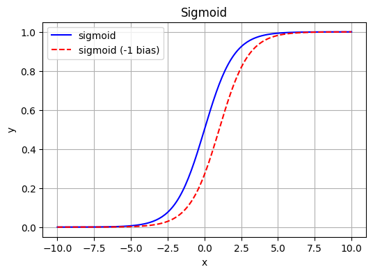
A common technique to shift a function curve left or right is to add a (constant) value to its input, known as a “bias”.
To illustrate, consider the sigmoid function (in blue). Normally, for x = 0, y = 1. By adding a bias of -1, we shift the function to the right, now for x = 0, y = 0.27 (which is just sigmoid(-1), in red).
Don’t worry about the sigmoid function for now, it will be introduced later on this article.
Step function
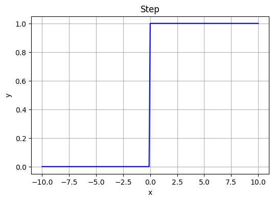
After computing the weighted sum, we pass the values to the step function:
- for x < 0, y = 0
- for x >= 0, y = 1
It essentially works as an on/off switch, off when negative and on when positive.
NOT gate
| a | NOT a |
|---|---|
| 0 | 1 |
| 1 | 0 |
The NOT gate that inverts the value.
Using the perceptron algorithm we discussed earlier (weighted sum, bias, and step function), we can implement the NOT gate with a single weight and bias.
def dot(vector1, vector2):
    return sum(x * y for x, y in zip(vector1, vector2))

def step(x):
    return 1 if x >= 0 else 0

def compute_perceptron(weights, bias, input):
    return step(dot(weights, input) + bias)

def compute_not(value):
    not_weights = [-2.]
    not_bias = 1.
    return compute_perceptron(not_weights, not_bias, [value])

print(f'NOT 0: {compute_not(0)}') # prints NOT 0: 1
print(f'NOT 1: {compute_not(1)}') # prints NOT 1: 0
AND and OR gates
| a | b | a AND b | a OR b |
|---|---|---|---|
| 0 | 0 | 0 | 0 |
| 0 | 1 | 0 | 1 |
| 1 | 0 | 0 | 1 |
| 1 | 1 | 1 | 1 |
Using a couple of weights and a bias, we can compute AND and OR gates.
def dot(vector1, vector2):
    return sum(x * y for x, y in zip(vector1, vector2))

def step(x):
    return 1 if x >= 0 else 0

def compute_perceptron(weights, bias, input):
    return step(dot(weights, input) + bias)

def compute_and(value_a, value_b):
    and_weights = [2., 2.]
    and_bias = -3.
    return compute_perceptron(and_weights, and_bias, [value_a, value_b])

def compute_or(value_a, value_b):
    or_weights = [2., 2.]
    or_bias = -1.
    return compute_perceptron(or_weights, or_bias, [value_a, value_b])

print(f'0 AND 0: {compute_and(0, 0)}') # prints 0 AND 0: 0
print(f'0 AND 1: {compute_and(0, 1)}') # prints 0 AND 1: 0
print(f'1 AND 0: {compute_and(1, 0)}') # prints 1 AND 0: 0
print(f'1 AND 1: {compute_and(1, 1)}') # prints 1 AND 1: 1
print()
print(f'0 OR 0: {compute_or(0, 0)}') # prints 0 OR 0: 0
print(f'0 OR 1: {compute_or(0, 1)}') # prints 0 OR 1: 1
print(f'1 OR 0: {compute_or(1, 0)}') # prints 1 OR 0: 1
print(f'1 OR 1: {compute_or(1, 1)}') # prints 1 OR 1: 1
XOR gate
| a | b | a XOR b |
|---|---|---|
| 0 | 0 | 0 |
| 0 | 1 | 1 |
| 1 | 0 | 1 |
| 1 | 1 | 0 |
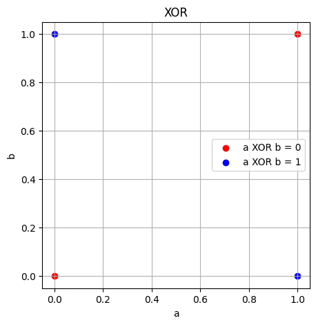
Unlike the other logic gates, the XOR gate is not linearly separable, that is, we cannot draw a single line to separate the outputted true values from the outputted false. As a result, a single perceptron cannot implement the XOR gate, a challenge known as “the XOR problem”.
Notice how the blue and red dots on the graph below cannot be separated by a single line.
Neural network
A single perceptron cannot compute the XOR gate because it is a non-linear function. However, by using more than one neuron and stacking them in layers, we can create what is called an “artificial neural network”.
Below is the structure of the neural network that we will implement in this article.
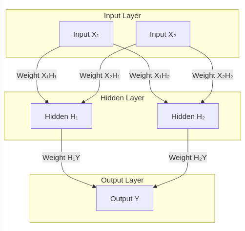
A typical neural network consists of an input layer, followed by one or more hidden layers, and an output layer.
In the neural network we are building to compute the XOR logic gate, the input layer has two neurons corresponding to the two inputs of the XOR gate, and the output layer has one neuron, reflecting the single output of the gate. The hidden layer contains two neurons, which is the minimum number required to solve the XOR problem.
Neural networks can have hidden layers of varying sizes. When a network has multiple hidden layers, it is referred to as a “deep” network. In this “feed-forward” network, the input propagates in a single direction, from the input layer to the output layer. Additionally, because each neuron in one layer is connected to every neuron in the subsequent layer, the network is termed “fully connected” or “dense”.
Each neuron typically includes an adjustable bias term (added to the summation of inputs), which is essential for shifting the activation function. However, for simplicity, biases are omitted from this diagram.
Sigmoid function
Before tackling the XOR problem, we are introducing a key change: instead of using the step function after calculating the weighted sum of inputs and biases, we will use the sigmoid function.
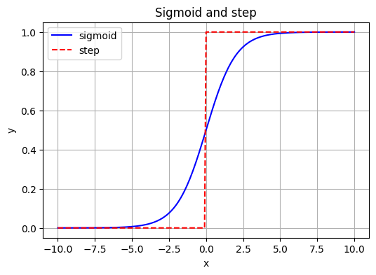
Observe in the plot below that both the sigmoid and step functions transition from 0 to 1. However, the key difference is that the sigmoid function provides a smooth, gradual transition, unlike the abrupt change seen in the step function.
The sigmoid function is an example of an “activation function”, which determines whether or not a neuron is activated based on its output.
Solving the XOR problem
Lastly, let’s build our neural network and manually set the weights that we know in advance will allow the network to solve the XOR problem.
from math import exp

def dot(vector1, vector2):
    return sum(x * y for x, y in zip(vector1, vector2))

def sigmoid(x):
    return 1 / (1 + exp(-x))

def compute_neuron(weights, inputs):
    bias = [1] # for this example we'll use a constant bias of 1
    input_with_bias = inputs + bias # making a list with inputs and bias
    return sigmoid(dot(weights, input_with_bias))

def compute_network(layers, input):
    outputs = []

    for layer in layers:
        output = [compute_neuron(neuron_weights, input) for neuron_weights in layer]
        outputs.append(output)
        input = output

    return outputs

def compute_xor(value_a, value_b):
    layers = [

        # hidden layer
        [[20., 20., -30], [20., 20., -10.]],

        # output layer
        [[-60., 60., -30.]]

    ]

    outputs = compute_network(layers, [value_a, value_b])
    last_output = outputs[-1][0]

    return round(last_output)

print(f'0 XOR 0: {compute_xor(0, 0)}') # prints 0 XOR 0: 0
print(f'0 XOR 1: {compute_xor(0, 1)}') # prints 0 XOR 1: 1
print(f'1 XOR 0: {compute_xor(1, 0)}') # prints 1 XOR 0: 1
print(f'1 XOR 1: {compute_xor(1, 1)}') # prints 1 XOR 1: 0
We’ve successfully built a neural network to solve the XOR problem, demonstrating how adding layers and using the right activation functions can tackle non-linear challenges.
This shows how even simple neural networks can handle tricky problems, paving the way for more complex applications.
Sources
- Weights values taken from “Data Science from Scratch”
- Electronic ‘Brain’ Teaches Itself (1958)
